1.TCGA RNA-seq数据更新情况
2022年3月29日,GDC官网(https://portal.gdc.cancer.gov/)发布了新的更新版本(Data Release 32.0)数据。此次数据更新范围广、变化大,导致许多网上的教程一夜之间不再直接可用。
具体的更新情况,在官网页面(https://docs.gdc.cancer.gov/Data/Release_Notes/Data_Release_Notes/)有详细介绍。对于应用最为广泛的RNA-seq数据,主要变化有:
- 测序数据比对注释的基因组版本更新 了,从GENECODE v22更新到了v36版本;
- 不同格式(Counts、FPKM、FPKM-UQ、TPM)的RNA-seq数据不再分为数个单独的文件,而是 同个样本的多种格式数据存储于同一个文件 ;
- 数据文件的格式 从txt格式改为了 tsv格式 ;
- 数据表格中 直接匹配了基因ID、基因名和基因类别信息 ,无需单独再从注释文件中提取;
- Counts数据 提供了Non-stranded Counts和Stranded Counts数据 。
Non-stranded RNA-Seq与Stranded RNA-seq的建库方法有所不同,有文献(DOI: 10.1186/s12864-015-1876-7)分析认为Stranded RNA-seq 得到的mRNA数据更为准确。
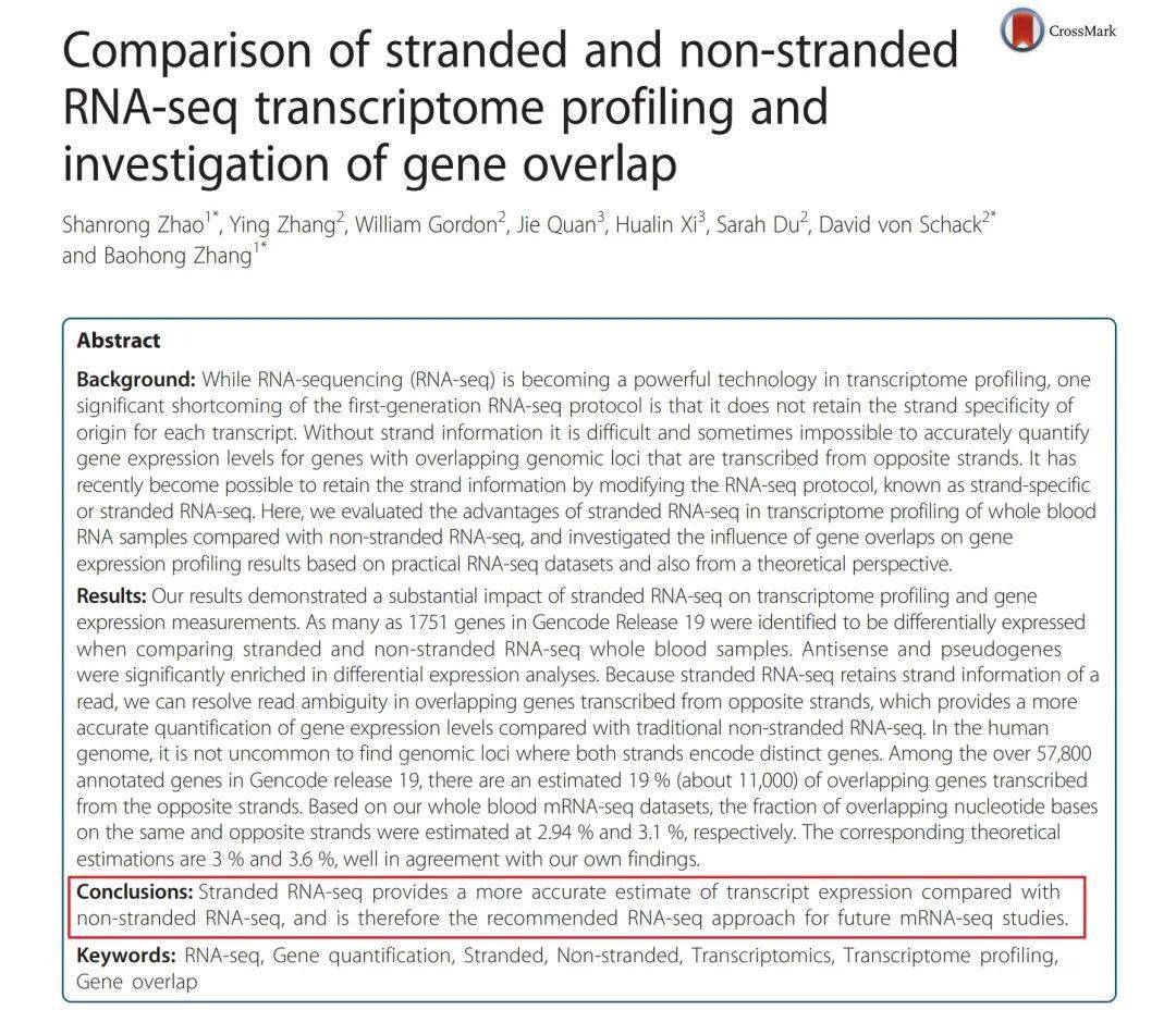
但是,对于大多数的分析来说,Non-stranded RNA-Seq数据用于常规分析已经足够(https://web.azenta.com/stranded-vs-non-stranded-rna-seq)。
Stranded RNA-Seq is strongly recommended if you’re trying to accomplish one or more of the following, as it’s important to capture information about tran directionality:
Identify antisense trans
Annotate a genome
Discover novel trans
Non-stranded RNA-Seq, on the other hand, is often sufficient for measuring gene expression in organisms with well-annotated genomes.
2. 更新后的TCGA RNA-seq数据的下载与读取
数据更新后,一些既往常用的数据下载和读取方法有所变化,本着“喂(bu)饭(yan)到(qi)口(fan)”的分享精神,此次我们重点介绍2种主要的数据下载和读取方法供大家享用。
2.1应用R包TCGAbiolinks下载和读取TCGA RNA-seq数据
TCGAbiolinks是一个常用的强大的检索、下载和预处理 The National Cancer Institute (NCI) Genomic Data Commons (GDC)数据的R包。如若使用该包,需引用相关的文献:
If you use TCGAbiolinks, please cite:
Colaprico, Antonio, et al. “TCGAbiolinks: an R/Bioconductor package for integrative analysis of TCGA data.” Nucleic acids research 44.8 (2015): e71-e71.
Silva, Tiago C., et al. “TCGA Workflow: Analyze cancer genomics and epigenomics data using Bioconductor packages.” F1000Research 5 (2016). (https://f1000research.com/articles/5-1542/v2)
Mounir, Mohamed, et al. “New functionalities in the TCGAbiolinks package for the study and integration of cancer data from GDC and GTEx.” PLoS computational biology 15.3 (2019): e1006701. (https://doi.org/10.1371/journal.pcbi.1006701)
GDC数据更新不到一个月后,TCGAbiolinks包就出了相应的更新版本处理数据下载和读取问题。
首先,需要安装该包的最新版本或开发版本。
-
安装最新的stable版本
if(!requireNamespace( "BiocManager", quietly= TRUE))
install.packages( "BiocManager") # BiocManager::install("TCGAbiolinks", force = TRUE) # 若未安装最新的版本,请选中运行上行代码
-
安装开发版本
if(!requireNamespace( "BiocManager", quietly = TRUE))
install.packages( "BiocManager") # BiocManager::install("BioinformaticsFMRP/TCGAbiolinksGUI.data")# BiocManager::install("BioinformaticsFMRP/TCGAbiolinks")# 若安装开发版本,请选中运行上两行代码
library(TCGAbiolinks)
1.2.1 R包TCGAbiolinks下载TCGA RNA-seq数据
使用TCGAbiolinks处理数据,常规需要3步走,分别是检索、下载和读取数据,依次对应以下3个函数 GDCquery、GDCdownload 和 GDCprepare 。
-
检索需要下载的数据
GDCquery可以通过多个参数检索限定需要下载的数据,各参数的详细说明可参阅帮助文档。此处,以样本量较少的ACC数据集为例。对于TCGA RNA-seq数据来说,一般仅需更改project参数即可。
query <- GDCquery(project = "TCGA-ACC",
data.category = "Tranome Profiling",
data.type = "Gene Expression Quantification",
workflow.type = "STAR - Counts")
-
下载检索的数据 如不设置特定的存储文件夹,TCGAbiolins下载的数据会在工作目录下新建一个名为GDCdata的文件夹用来存储下载的数据文件,数据有特定的命名和组织形式。下载数据仅需在前述query的基础上一行代码搞定,速度快慢取决于文件大小和网络情况。
# 若文件夹中已下载,可掠过此步骤GDCdownload(query)
1.2.2 R包TCGAbiolinks读取TCGA RNA-seq数据
-
读取下载的数据
data <- GDCprepare(query)
##
| | 0%
| |1.265823% ~3 s remaining
|= |2.531646% ~2 s remaining
|= |3.797468% ~2 s remaining
|== |5.063291% ~2 s remaining
|=== |6.329114% ~2 s remaining
|=== |7.594937% ~2 s remaining
|==== |8.860759% ~2 s remaining
|===== |10.12658% ~5 s remaining
|===== |11.39241% ~4 s remaining
|====== |12.65823% ~4 s remaining
|======= |13.92405% ~4 s remaining
|======= |15.18987% ~4 s remaining
|======== |16.4557% ~3 s remaining
|========= |17.72152% ~3 s remaining
|========= |18.98734% ~3 s remaining
|========== |20.25316% ~3 s remaining
|=========== |21.51899% ~4 s remaining
|=========== |22.78481% ~4 s remaining
|============ |24.05063% ~4 s remaining
|============= |25.31646% ~3 s remaining
|============= |26.58228% ~3 s remaining
|============== |27.8481% ~3 s remaining
|=============== |29.11392% ~3 s remaining
|=============== |30.37975% ~3 s remaining
|================ |31.64557% ~3 s remaining
|================= |32.91139% ~3 s remaining
|================= |34.17722% ~3 s remaining
|================== |35.44304% ~3 s remaining
|=================== |36.70886% ~3 s remaining
|=================== |37.97468% ~3 s remaining
|==================== |39.24051% ~3 s remaining
|===================== |40.50633% ~3 s remaining
|===================== |41.77215% ~2 s remaining
|====================== |43.03797% ~2 s remaining
|======================= |44.3038% ~2 s remaining
|======================= |45.56962% ~2 s remaining
|======================== |46.83544% ~2 s remaining
|========================= |48.10127% ~2 s remaining
|========================= |49.36709% ~2 s remaining
|========================== |50.63291% ~2 s remaining
|========================== |51.89873% ~2 s remaining
|=========================== |53.16456% ~2 s remaining
|============================ |54.43038% ~2 s remaining
|============================ |55.6962% ~2 s remaining
|============================= |56.96203% ~2 s remaining
|============================== |58.22785% ~2 s remaining
|============================== |59.49367% ~2 s remaining
|=============================== |60.75949% ~2 s remaining
|================================ |62.02532% ~2 s remaining
|================================ |63.29114% ~1 s remaining
|================================= |64.55696% ~1 s remaining
|================================== |65.82278% ~1 s remaining
|================================== |67.08861% ~1 s remaining
|=================================== |68.35443% ~1 s remaining
|==================================== |69.62025% ~1 s remaining
|==================================== |70.88608% ~1 s remaining
|===================================== |72.1519% ~1 s remaining
|====================================== |73.41772% ~1 s remaining
|====================================== |74.68354% ~1 s remaining
|======================================= |75.94937% ~1 s remaining
|======================================== |77.21519% ~1 s remaining
|======================================== |78.48101% ~1 s remaining
|========================================= |79.74684% ~1 s remaining
|========================================== |81.01266% ~1 s remaining
|========================================== |82.27848% ~1 s remaining
|=========================================== |83.5443% ~1 s remaining
|============================================ |84.81013% ~1 s remaining
|============================================ |86.07595% ~1 s remaining
|============================================= |87.34177% ~0 s remaining
|============================================== |88.60759% ~0 s remaining
|============================================== |89.87342% ~0 s remaining
|=============================================== |91.13924% ~0 s remaining
|================================================ |92.40506% ~0 s remaining
|================================================ |93.67089% ~0 s remaining
|================================================= |94.93671% ~0 s remaining
|================================================== |96.20253% ~0 s remaining
|================================================== |97.46835% ~0 s remaining
|=================================================== |98.73418% ~0 s remaining
|====================================================|100% ~0 s remaining
|====================================================|100% Completed after 4 s
data数据是以SummarizedExperiment class格式组织的,此类数据对象的详细介绍请参阅https://bioconductor.org/help/course-materials/2019/BSS2019/04_Practical_CoreApproachesInBioconductor.html。
SummarizedExperiment数据的组织形式示意图如下:
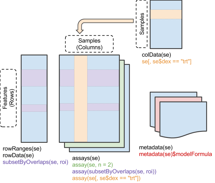
该data数据中同时包含了多种不同格式的RNA-seq数据,可以使用assayNames函数查看包含的数据名称。主要包含以下几种,依次对应index 1-6。
[1] “unstranded” “stranded_first” “stranded_second”
[4} “tpm_unstrand” “fpkm_unstrand” “fpkm_uq_unstrand”
library(SummarizedExperiment)
assayNames(data)
## [1] "unstranded" "stranded_first" "stranded_second" "tpm_unstrand"
## [5] "fpkm_unstrand" "fpkm_uq_unstrand"
设置不同不同的index参数,可对应提取不同格式的表达矩阵数据。
data_counts <- assay(data, i = 1)
data_counts_first <- assay(data, i = 2)
data_counts_second <- assay(data, i = 3)
data_tpm <- assay(data, i = 4)
data_fpkm <- assay(data, i = 5)
data_fpkm_uq <- assay(data, i = 6)
head(data_counts)[, 1: 2]
## TCGA-OR-A5JD-01A-11R-A29S-07 TCGA-OR-A5L5-01A-11R-A29S-07
## ENSG00000000003.15 2086 3813
## ENSG00000000005.6 2 3
## ENSG00000000419.13 2086 2909
## ENSG00000000457.14 300 476
## ENSG00000000460.17 79 135
## ENSG00000000938.13 110 374
data数据对象中还包含了基因注释信息和样本、临床信息,可分别通过rowData、colData函数提取。
rowdata <- rowData(data)
coldata <- colData(data)
2.2直接从GDC官网下载和读取TCGA RNA-seq数据
简要介绍完使用TCGAbiolinks下载和读取更新后的RNA-seq数据,接着我们介绍一下如何直接从GDC官网直接下载和在R中读取数据。
2.2.1 从GDC官网下载下载TCGA RNA-seq数据
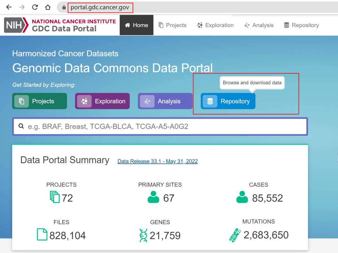
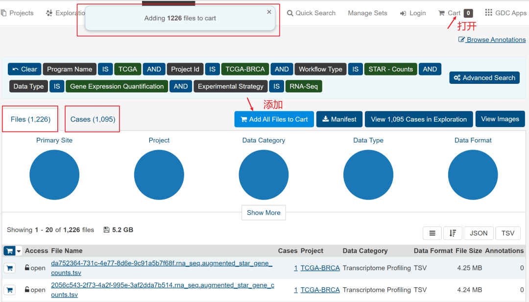
进入GDC Data Portal主页https://portal.gdc.cancer.gov/,见到如下图页面,点击Repository。
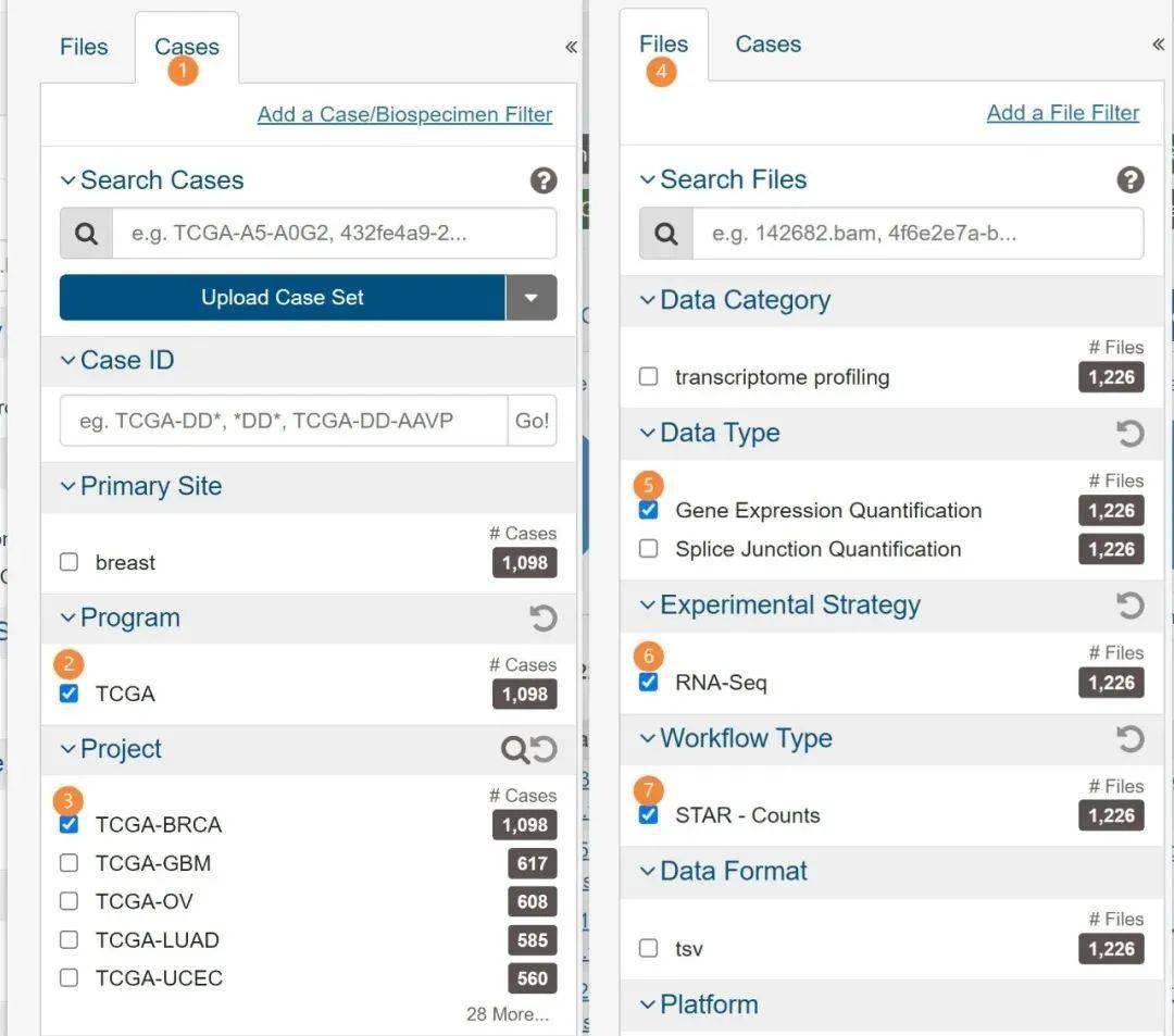
以TCGA中样本样本数最多的BRCA数据集为例,有1226个样本,如果这个数据集可以处理好,其他的数据集应该都不成问题。分别按顺序点击或勾选下图中标记的地方。
然后,如下图,点击额右侧的Add All Files to Cart,然后进入Cart。
见到下图,离数据下载好就一步之遥了。
需要下载的有3个文件,分别是数据文件、样本信息文件和临床信息文件。如下图所标记。
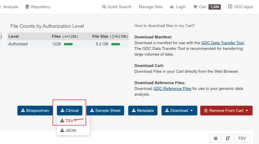
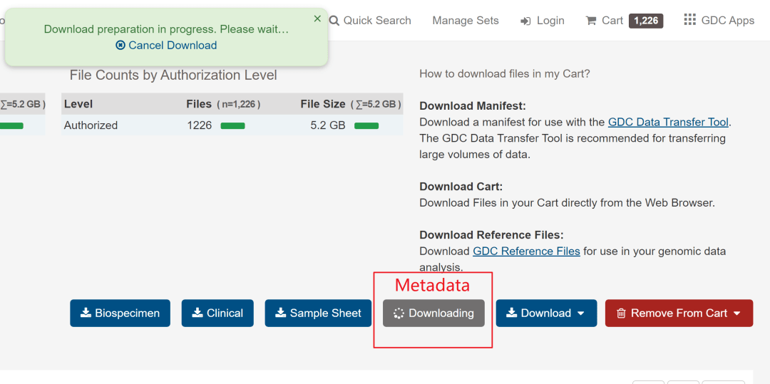
第3个需要下载的是数据文件,比较大,但直接点击Cart下载就好,也不算太耗时,下载的所有文件会在一个压缩文件里,然后解压到文件夹内。
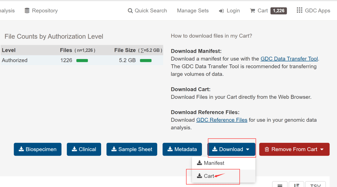
中间会提示推荐使用工具下载,不要取消,忽略就行,等待弹出窗口(等待时间可能与网速有关)。我这大致按照下图的速度下载,下载完成差不多15分钟,压缩文件大小1.18G,解压后4.84G,比使用GDC Data Transfer Tool工具下载还是快很多的。
下载完成,然后在Rstudio里新建一个Rproject文件和R代码文件。文件夹内一共有以下7个文件。就可以开始在R中用代码读取了(临床信息文件此次暂时用不上,但后面大概率会用到)。
2.2.2 R中读取手动下载的TCGA RNA-seq数据
点击BRCA.Proj文件进入Rstudio,工作目录就自然在上述文件所在的文件夹,打开.R代码文件,正式开始读取。
-
加载相关的R包
library(tidyverse) # 数据清洗与读取的利器library(vroom) # vroom可以快速读取tsv文件library(jsonlite) # 读取metadata文件library(tictoc) # 计时器
-
事先设置VROOM读取文件的参数
Sys.setenv( "VROOM_CONNECTION_SIZE"= 10^ 6)
-
metadata 信息提取函数 这个函数可以方便快捷地提取下载的json格式的metadata文件内的有用信息。函数代码如下,运行代码之后,就可以使用了。此处不再逐行解释。
TCGA_metadata <- function(path = json_file) {
metadata <- jsonlite::read_json(path, simplifyVector = T)
metadata <- tibble::tibble(
file_name = metadata$file_name,
md5sum = metadata$md5sum,
TCGA_id_full = bind_rows(metadata$associated_entities)$entity_submitter_id,
TCGA_id = stringr::str_sub(TCGA_id_full, 1, 16),
patient_id = stringr::str_sub(TCGA_id, 1, 12),
tissue_type_id = stringr::str_sub(TCGA_id, 14, 15),
tissue_type = sapply(tissue_type_id, function(x) { switch(x, "01"= "Primary Solid Tumor", "02"= "Recurrent Solid Tumor", "03"= "Primary Blood Derived Cancer - Peripheral Blood", "05"= "Additional - New Primary", "06"= "Metastatic", "07"= "Additional Metastatic", "11"= "Solid Tissue Normal")}),
group = ifelse(tissue_type_id == "11", "Normal", "Tumor")) return(metadata)
}
有了上面的函数,一行代码提取metadata的信息。
metadata <- TCGA_metadata(path = "metadata.cart.2022-06-05.json")
head(metadata)
## # A tibble: 6 x 8
## file_name md5sum TCGA_id_full TCGA_id patient_id tissue_type_id tissue_type
## <chr> <chr> <chr> <chr> <chr> <chr> <chr>
## 1 da752364-73~ 6f358~ TCGA-E2-A1L~ TCGA-E~ TCGA-E2-A~ 11 Solid Tiss~
## 2 2056c543-2f~ 6a9b5~ TCGA-E2-A1L~ TCGA-E~ TCGA-E2-A~ 01 Primary So~
## 3 90950125-1b~ ca15f~ TCGA-AR-A0U~ TCGA-A~ TCGA-AR-A~ 01 Primary So~
## 4 48c63209-a3~ f0c8e~ TCGA-BH-A28~ TCGA-B~ TCGA-BH-A~ 01 Primary So~
## 5 824f5b0a-44~ 5a849~ TCGA-A2-A0D~ TCGA-A~ TCGA-A2-A~ 01 Primary So~
## 6 a8e0466b-d1~ f5542~ TCGA-E9-A1R~ TCGA-E~ TCGA-E9-A~ 01 Primary So~
## # ... with 1 more variable: group <chr>
-
把要读取的tsv文件的完整路径加入到上面的metadata数据中,并且一一对应。
tsv_files <- list.files(path = ".",
pattern = "counts.tsv",
full.names = T,
recursive = T)
-
新metadata数据
metadata <- metadata %>%
left_join(y = tibble(file_name = basename(tsv_files), tsv_files))
## Joining, by = "file_name"
TCGA的基因注释信息
id2symbol <- vroom::vroom(tsv_files[ 1], # 读取第一个文件
col_select = 1: 3, # 只选择前3列读取
comment = "#", # 设置注释符号
skip = 5, #前5行信息不需要,跳过
show_col_types = FALSE) %>% # 隐藏提示信息
set_names( "gene_id", "gene_name", "gene_type") # 设置列名head(id2symbol) # 查看数据
## # A tibble: 6 x 3
## gene_id gene_name gene_type
## <chr> <chr> <chr>
## 1 ENSG00000000003.15 TSPAN6 protein_coding
## 2 ENSG00000000005.6 TNMD protein_coding
## 3 ENSG00000000419.13 DPM1 protein_coding
## 4 ENSG00000000457.14 SCYL3 protein_coding
## 5 ENSG00000000460.17 C1orf112 protein_coding
## 6 ENSG00000000938.13 FGR protein_coding
-
读取以及合并 tsv files
这部分是最主要的代码块,关键在map_dfc函数。如若有不了解的地方,可以查看一下相关函数的说明文档。vroom函数里设置col_select = 4,读取的就是counts数据,其他数字对应的数据格式,如下图。
tic
counts_df <- map_dfc(.x = metadata$tsv_files,
.f = ~ vroom::vroom(.x,
col_select = 4,
comment = "#",
skip = 5,
show_col_types = FALSE,
progress = F,
.name_repair = "minimal")
) %>%
set_names(metadata$TCGA_id_full) %>%
bind_cols(id2symbol[ , "gene_id"], .)
toc
## 19.66 sec elapsed
# 23.5 sec elapsed 我的电脑上不到半分钟搞定数据读取与合并head(counts_df)[ 1: 3]
## # A tibble: 6 x 3
## gene_id `TCGA-E2-A1L7-11A-33R-A144-07` `TCGA-E2-A1L7-01A-11R-A144~`
## <chr> <dbl> <dbl>
## 1 ENSG00000000003.15 4209 1689
## 2 ENSG00000000005.6 71 16
## 3 ENSG00000000419.13 1611 1810
## 4 ENSG00000000457.14 1217 1098
## 5 ENSG00000000460.17 346 715
## 6 ENSG00000000938.13 787 624
到此,数据读取与合并就完成了。
sessionInfo
## R version 4.1.1 (2021-08-10)
## Platform: x86_64-w64-mingw32/x64 (64-bit)
## Running under: Windows 10 x64 (build 19043)
##
## Matrix products: default
##
## locale:
## [1] LC_COLLATE=Chinese (Simplified)_China.936
## [2] LC_CTYPE=Chinese (Simplified)_China.936
## [3] LC_MONETARY=Chinese (Simplified)_China.936
## [4] LC_NUMERIC=C
## [5] LC_TIME=Chinese (Simplified)_China.936
##
## attached base packages:
## [1] parallel stats4 stats graphics grDevices utils datasets
## [8] methods base
##
## other attached packages:
## [1] tictoc_1.0.1 jsonlite_1.8.0
## [3] vroom_1.5.7 forcats_0.5.1
## [5] stringr_1.4.0 dplyr_1.0.9
## [7] purrr_0.3.4 readr_2.1.2
## [9] tidyr_1.2.0 tibble_3.1.7
## [11] ggplot2_3.3.6 tidyverse_1.3.1
## [13] SummarizedExperiment_1.22.0 Biobase_2.52.0
## [15] GenomicRanges_1.44.0 GenomeInfoDb_1.28.4
## [17] IRanges_2.26.0 S4Vectors_0.30.2
## [19] BiocGenerics_0.38.0 MatrixGenerics_1.4.3
## [21] matrixStats_0.62.0 TCGAbiolinks_2.25.0
##
## loaded via a namespace (and not attached):
## [1] fs_1.5.2 bitops_1.0-7
## [3] lubridate_1.8.0 bit64_4.0.5
## [5] filelock_1.0.2 progress_1.2.2
## [7] httr_1.4.3 backports_1.4.1
## [9] tools_4.1.1 bslib_0.3.1
## [11] utf8_1.2.2 R6_2.5.1
## [13] DBI_1.1.2 colorspace_2.0-3
## [15] withr_2.5.0 tidyselect_1.1.2
## [17] prettyunits_1.1.1 bit_4.0.4
## [19] curl_4.3.2 compiler_4.1.1
## [21] cli_3.1.0 rvest_1.0.2
## [23] xml2_1.3.3 DelayedArray_0.18.0
## [25] sass_0.4.1 scales_1.2.0
## [27] rappdirs_0.3.3 digest_0.6.29
## [29] rmarkdown_2.14 XVector_0.32.0
## [31] pkgconfig_2.0.3 htmltools_0.5.2
## [33] dbplyr_2.1.1 fastmap_1.1.0
## [35] readxl_1.4.0 rlang_1.0.2
## [37] rstudioapi_0.13 RSQLite_2.2.14
## [39] jquerylib_0.1.4 generics_0.1.2
## [41] RCurl_1.98-1.6 magrittr_2.0.3
## [43] GenomeInfoDbData_1.2.6 Matrix_1.4-1
## [45] Rcpp_1.0.8.3 munsell_0.5.0
## [47] fansi_1.0.3 lifecycle_1.0.1
## [49] stringi_1.7.6 yaml_2.3.5
## [51] zlibbioc_1.38.0 plyr_1.8.7
## [53] BiocFileCache_2.0.0 grid_4.1.1
## [55] blob_1.2.3 crayon_1.5.1
## [57] lattice_0.20-45 haven_2.5.0
## [59] Biostrings_2.60.2 hms_1.1.1
## [61] KEGGREST_1.32.0 knitr_1.39
## [63] pillar_1.7.0 TCGAbiolinksGUI.data_1.15.1
## [65] biomaRt_2.48.3 reprex_2.0.1
## [67] XML_3.99-0.9 glue_1.6.2
## [69] evaluate_0.15 downloader_0.4
## [71] modelr_0.1.8 data.table_1.14.2
## [73] BiocManager_1.30.18 png_0.1-7
## [75] vctrs_0.4.1 tzdb_0.3.0
## [77] cellranger_1.1.0 gtable_0.3.0
## [79] assertthat_0.2.1 cachem_1.0.6
## [81] xfun_0.31 broom_0.8.0
## [83] AnnotationDbi_1.54.1 memoise_2.0.1
## [85] ellipsis_0.3.2
— END—
转自解螺旋生信频道-挑圈联靠公号- 本文固定链接: https://maimengkong.com/zu/1538.html
- 转载请注明: : 萌小白 2023年5月14日 于 卖萌控的博客 发表
- 百度已收录