2020年4分+甲基化生信文章复现
领悟生信文章逻辑之美,小伙伴们大家好呀,我是风间琉璃。上一周我们品读了2020年10月发表在《Frontiers in oncology》杂志上的文章“ A Novel Promoter CpG-Based Signature for Long-Term Survival Prediction of Breast Cancer Patients”。作者使用CHAMP包进行筛选差异的甲基化位点。还没看上一期推文的同学们请看一遍,看过的同学可以复习一遍。“ 2020年了!!这样的文章也能发近5分! ”。因为接下来我们会使用CHAMP包来适当复现文章中的流程。很精彩,不要错过喔~
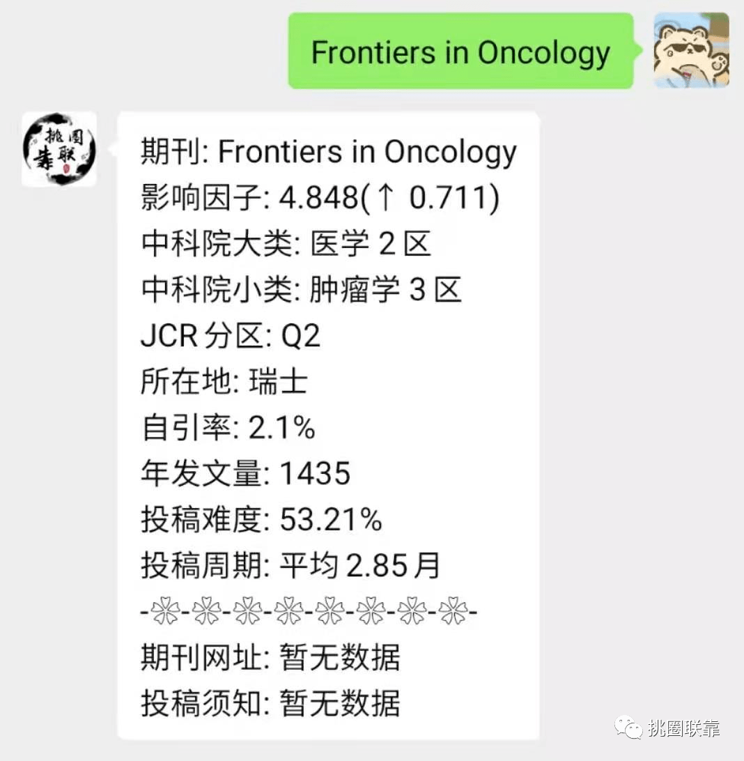
期刊信息
下载数据
首先我们需要下载相关的甲基化数据以及表型(phenotype)数据。进入xena官网(https://xena.ucsc.edu/),选择数据集进行下载。如果不想自己找的同学没关系,我提供了下载地址。乳腺癌甲基化数据集下载链接(https://xenabrowser.net/datapages/?dataset=TCGA-BRCA.methylation450.tsv&host=https%3A%2F%2Fgdc.xenahubs.net&removeHub=https%3A%2F%2Fxena.treehouse.gi.ucsc.edu%3A443)。表型数据下载链接(https://xenabrowser.net/datapages/?dataset=TCGA-BRCA.GDC_phenotype.tsv&host=https%3A%2F%2Fgdc.xenahubs.net&removeHub=https%3A%2F%2Fxena.treehouse.gi.ucsc.edu%3A443)。
数据读取及数据清洗
在读取之前注意,我们R语言的工作路径一定要和我们文件的目录一致,才能进行以下步骤。
#加载数据 library(tidyverse) data_beta=read_tsv(file = "TCGA-BRCA.methylation450.tsv") data_samp=read_tsv(file = "phenotype.tsv")
读取数据之后,我们需要对数据进行初步清洗。
###查看甲基化数据和表型数据的维度和数据格式 dim(data_beta) ## [1] 485577 891 dim(data_samp) ## [1] 1284 140 class(data_beta) ## [1] "spec_tbl_df" "tbl_df" "tbl" "data.frame" class(data_samp) ## [1] "spec_tbl_df" "tbl_df" "tbl" "data.frame" ######提取肿瘤和正常样本的信息 table(data_samp$sample_type.samples) ## ## Metastatic Primary Tumor Solid Tissue Normal ## 7 1114 162 ##我们只要"Primary Tumor"和"Solid Tissue Normal" tissue=c( "Primary Tumor", "Solid Tissue Normal") data_samp=data_samp[data_samp$sample_type.samples%in%tissue,] ###提取病人编号和样本信息 pdata=data_samp[,c( "submitter_id.samples", "sample_type.samples")] ###接下来具有甲基化数据和表型数据之间需要对病人信息取交集 ID=intersect(pdata$submitter_id.samples, colnames(data_beta)) ##一共885个样本,文章提示一共为890个样本,疾病组794个,正常组96个。看一下我们 ##自己的,正常样本96没问题,肿瘤组织789个,少了5个,关系不大。 #提取具有共同交集的sample信息 pdata=pdata[pdata$submitter_id.samples%in%ID,] #查看整理好的表型数据 dim(pdata) ## [1] 885 2 #更改一下表型数据的列名,并把结果输出为data_samp数据 names(pdata) <- c( "sample_name", "sample_group") data_samp <- pdata #提取具有共同交集的beta矩阵 names(data_beta)[1]= "CpG" data_beta=column_to_rownames(data_beta, "CpG") data_beta=data_beta[,ID] ####清洁数据不易,记得保存 save(data_beta,data_samp,file = "methylation.rds")
接下来,我们需要开始将清洁数据导入CHAMP包中。
数据导入
#加载数据和包 library(ChAMP) library(tidyverse) ## ── Attaching packages ─────────────────────────────────────── tidyverse 1.3.0 ── ## ✓ ggplot2 3.3.2 ✓ purrr 0.3.4 ## ✓ tibble 3.0.4 ✓ dplyr 1.0.2 ## ✓ tidyr 1.1.2 ✓ stringr 1.4.0 ## ✓ readr 1.4.0 ✓ forcats 0.5.0 ## ── Conflicts ────────────────────────────────────────── tidyverse_conflicts ── ## x purrr::accumulate masks foreach::accumulate ## x dplyr::collapse masks Biostrings::collapse, IRanges::collapse ## x dplyr::combine masks minfi::combine, Biobase::combine, BiocGenerics::combine ## x purrr::compact masks XVector::compact ## x dplyr::count masks matrixStats::count ## x dplyr::desc masks IRanges::desc ## x tidyr::expand masks S4Vectors::expand ## x dplyr::filter masks stats::filter ## x dplyr::first masks S4Vectors::first ## x dplyr::lag masks stats::lag ## x purrr::none masks locfit::none ## x ggplot2::Position masks BiocGenerics::Position, base::Position ## x purrr::reduce masks GenomicRanges::reduce, IRanges::reduce ## x dplyr::rename masks S4Vectors::rename ## x purrr::simplify masks DelayedArray::simplify ## x dplyr::slice masks XVector::slice, IRanges::slice ## x purrr::when masks foreach::when load("methylation.rds") ##增加一列Sample_Group,肿瘤组织为T,正常组织为C。方便后续差异分析 data_samp$Sample_Group <- if_else(data_samp $sample_group== "Primary Tumor", data_samp$Sample_Group <- "T", data_samp$Sample_Group <- "C") data_samp <- as.data.frame(data_samp) ###beta矩阵的处理 ##有以下几点,1.保持beta矩阵的列名和表型数据的样本名一致,这很重要! ##2.beta矩阵里不能有NA ##3.beta矩阵中最小值如果为0,可以加上0.00001防止报错 ##4.beta矩阵必须为矩阵数据格式 data_order=data_beta[,data_samp$sample_name] data_order=as.matrix(data_order) sum(is.na(data_order)) ## [1] 0 data_order=data_order+0.00001 ###CHAMP包导入 myLoad=champ.filter(beta = data_order,pd = data_samp) ## [===========================] ## [<<<< ChAMP.FILTER START >>>>>] ## ----------------------------- ## ## In New version ChAMP, champ.filter function
has been set to do filtering on the result of champ.import. You can use
champ.import + champ.filter to do Data Loading, or set "method"
parameter in champ.load as "ChAMP" to get the same effect. ## ## This function is provided for user need to
do filtering on some beta (or M) matrix, which contained most filtering
system in champ.load except beadcount. User need to input beta matrix,
pd file themselves. If you want to do filterintg on detP matrix and Bead
Count, you also need to input a detected P matrix and Bead Count
information. ## ## Note that if you want to filter more data
matrix, say beta, M, intensity... please make sure they have exactly the
same rownames and colnames. ## ## ## [ Section 1: Check Input Start ] ## You have inputed beta for Analysis. ## ## pd file provided, checking if it's in accord with Data Matrix... ## !!! Your pd file does not have Sample_Name column, we can not check your Sample_Name, please make sure the pd file is correct. ## ## Parameter filterDetP is TRUE, checking if detP in accord with Data Matrix... ## !!! Parameter detP is not found, filterDetP is reset FALSE now. ## ## Parameter filterBeads is TRUE, checking if beadcount in accord with Data Matrix... ## !!! Parameter beadcount is not found, filterBeads is reset FALSE now. ## ## parameter autoimpute is TRUE. Checking if the conditions are fulfilled... ## !!! ProbeCutoff is 0, which means you have no needs to do imputation. autoimpute has been reset FALSE. ## ## Checking Finished :filterMultiHit,filterSNPs,filterNoCG,filterXY would be done on beta. ## [ Section 1: Check Input Done ] ## ## ## [ Section 2: Filtering Start >> ## ## Filtering NoCG Start ## Only Keep CpGs, removing 3156 probes from the analysis. ## ## Filtering SNPs Start ## Using general 450K SNP list for filtering. ## Filtering probes with SNPs as identified in Zhou's Nucleic Acids Research Paper 2016. ## Removing 59901 probes from the analysis. ## ## Filtering MultiHit Start ## Filtering probes that align to multiple locations as identified in Nordlund et al ## Removing 11 probes from the analysis. ## ## Filtering XY Start ## Filtering probes located on X,Y chromosome, removing 10028 probes from the analysis. ## ## Updating PD file ## filterDetP parameter is FALSE, so no Sample Would be removed. ## ## Fixing Outliers Start ## Replacing all value smaller/equal to 0 with smallest positive value. ## Replacing all value greater/equal to 1 with largest value below 1.. ## [ Section 2: Filtering Done ] ## ## All filterings are Done, now you have 412481 probes and 885 samples. ## [<<<<< ChAMP.FILTER END >>>>>>] ## [===========================] ## [You may want to process champ.QC next.] ##成功导入后及时保存 #save(myLoad,file= "meth_load.rds") ###另外800多个病人,速度会比较慢。。。。 ###标准化,我们使用文章中使用的BMIQ法进行标准化。core值根据自己分析环境设置 #myNorm <- champ.norm(beta=myLoad $beta,arraytype= "450K",cores=100) ###同样及时保存,如果是自己的电脑就不要跑这一步了,会崩的,所以我就不演示了 #save(myNorm,file= "meth_norm.rds") ##标准化后得到新的数据 ##标准化后数据质控 #champ.QC ####甲基化差异位点分析 myDMP <- champ.DMP(beta = myLoad$beta ,pheno=myLoad$pd$Sample_Group) ## [===========================] ## [<<<<< ChAMP.DMP START >>>>>] ## ----------------------------- ## !!! Important !!! New Modification has been made on champ.DMP: ## (1): In this version champ.DMP if your pheno
parameter contains more than two groups of phenotypes, champ.DMP would
do pairewise differential methylated analysis between each pair of them.
But you can also specify compare.group to only do comparasion between
any two of them. ## (2): champ.DMP now support numeric as pheno,
and will do linear regression on them. So covariates like age could be
inputted in this function. You need to make sure your inputted "pheno"
parameter is "numeric" type. ## -------------------------------- ## ## [ Section 1: Check Input Pheno Start ] ## You pheno is character type. ## Your pheno information contains following groups. >> ## <T>:789 samples. ## <C>:96 samples. ## [The power of statistics analysis on groups contain very few samples may not strong.] ## pheno contains only 2 phenotypes ## compare.group parameter is NULL, two pheno types will be added into Compare List. ## T_to_C compare group : T, C ## ## [ Section 1: Check Input Pheno Done ] ## ## [ Section 2: Find Differential Methylated CpGs Start ] ## ----------------------------- ## Start to Compare : T, C ## Contrast Matrix ## Contrasts ## Levels pT-pC ## pC -1 ## pT 1 ## You have found 241364 significant MVPs with a BH adjusted P-value below 0.05. ## Calculate DMP for T and C done. ## ## [ Section 2: Find Numeric Vector Related CpGs Done ] ## ## [ Section 3: Match Annotation Start ] ## ## [ Section 3: Match Annotation Done ] ## [<<<<<< ChAMP.DMP END >>>>>>] ## [===========================] ## [You may want to process DMP.GUI or champ.GSEA next.] #查看我们的分析结果 head(myDMP[[1]]) ## logFC AveExpr t P.Value adj.P.Val B ## cg19533977 -0.3539830 0.1261480 -39.40782 8.157138e-197 3.364664e-191 439.1822 ## cg18269493 -0.3400004 0.1738861 -38.73995 1.171007e-192 2.415092e-187 429.6075 ## cg18265162 -0.2540523 0.1249706 -37.97257 7.378373e-188 1.014480e-182 418.5535 ## cg17046586 0.3694429 0.8027515 37.92441 1.478829e-187 1.524972e-182 417.8581 ## cg14789818 0.4325909 0.7772445 37.46889 1.073826e-184 8.858657e-180 411.2687 ## cg01393234 -0.3421082 0.1641259 -36.85815 7.573636e-181 5.206635e-176 402.4054 ## T_AVG C_AVG deltaBeta CHR MAPINFO Strand Type gene ## cg19533977 0.08774981 0.4417328 0.3539830 17 57719682 F II CLTC ## cg18269493 0.13700474 0.4770051 0.3400004 1 8772984 F II RERE ## cg18265162 0.09741234 0.3514647 0.2540523 1 210407588 R II C1orf133 ## cg17046586 0.84282668 0.4733838 -0.3694429 12 50665774 R II LIMA1 ## cg14789818 0.82416958 0.3915786 -0.4325909 1 227748712 R I ## cg01393234 0.12701586 0.4691241 0.3421082 1 226085079 F II ## feature cgi feat.cgi UCSC_CpG_Islands_Name DHS Enhancer ## cg19533977 Body opensea Body-opensea NA TRUE ## cg18269493 5'UTR opensea 5'UTR-opensea NA NA ## cg18265162 TSS200 island TSS200-island chr1:210407401-210407637 TRUE NA ## cg17046586 5'UTR opensea 5'UTR-opensea NA TRUE ## cg14789818 IGR island IGR-island chr1:227748423-227748860 NA NA ## cg01393234 IGR opensea IGR-opensea TRUE TRUE ## Phantom Probe_SNPs Probe_SNPs_10 ## cg19533977 ## cg18269493 ## cg18265162 ## cg17046586 ## cg14789818 ## cg01393234 ####差异甲基化区域,DMR #myDMR <- champ.DMR(beta=myLoad $beta,pheno=myLoad $pd$Sample_Group,method= "Bumphunter") #查看差异甲基化区域 #head(myDMR $BumphunterDMR)
接下来,根据文章中的条件进行筛选。
差异甲基化位点
文章中的条件筛选包括:
(1)adj.P<0.05,delta |β|>0.2
(2)位于启动子区域(5’-UTR, TSS200, TSS1500 and 1stExon),那我们开始把。
#提取我们得到的差异甲基化位点矩阵 feature_pro=c( "1stExon", "5'UTR", "TSS1500", "TSS200") data_dif <- myDMP[[ 1]] %>% filter(adj.P.Val< 0. 05& abs(deltaBeta)> 0. 2) data_dif <- data_dif[data_dif$feature%in%feature_pro,]
最后我们一共得到8778个位点,和作者的10088个差异甲基化位点有1000多个甲基化位点的差异,这可能是因为我们并没有做标准化这一步(数据量太大了,跑不了。。。。) 接下来我们绘制Figure 1B的热图。
复现热图
#加载包 library(pheatmap) #设置注释列名的文件ann_col ann_col <- data_samp ann_col$Sample_Group <- if_else(data_samp$sample_group== "Primary Tumor", data_samp$Sample_Group <- "Tumor", data_samp$Sample_Group <- "Normal") ann_col <- ann_col %>% column_to_rownames( var= "sample_name") %>% dplyr::select(-sample_group) %>%dplyr::select(-case_submitter_id) %>% arrange(Sample_Group) ##根据差异甲基化位点提取beta矩阵子集 data_heat=data_beta[rownames(data_dif),rownames(ann_col)] pheatmap(data_heat,color =colorRampPalette(c( "navy", "white",
"firebrick3"))( 10),cluster_rows = F,cluster_cols = F, legend = F,show_rownames = F,show_colnames = F,annotation_col = ann_col)
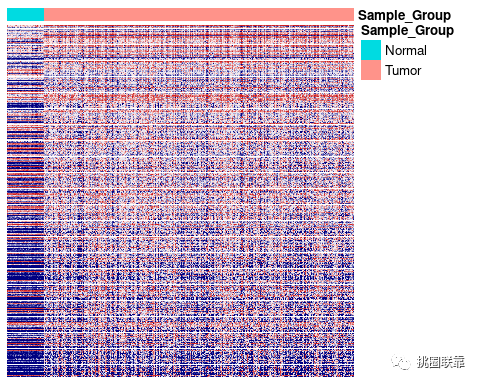
好啦,热图的复现差不多就结束了。
转自:挑圈联盟