分析代谢组数据，大名鼎鼎的xcms来了！

xcms是基于R语言设计的程序包(R package)，可以用分析代谢组数据等。下面我们就来介绍一下使用方法。

操作步骤

示例数据是fatty acid amide hydrolase (FAAH) 基因敲除鼠的脊柱LC-MS，六个基因敲除个体，六个野生型，使用的是centroid mode ，正离子模式，200-600 m/z ，2500-4500 seconds。

source("https://bioconductor.org/biocLite.R") yum install netcdf yum install netcdf-devel.x86_64 biocLite("xcms") biocLite("ncdf4") biocLite("faahKO") biocLite("MSnbase") library(xcms) library(faahKO) library(RColorBrewer) library(pander)

#读取数据

cdfs <- dir(system.file("cdf", package = "faahKO"), full.names = TRUE,recursive = TRUE) > cdfs [1] "C:/Program Files/R/R-3.4.2/library/faahKO/cdf/KO/ko15.CDF" "C:/Program Files/R/R-3.4.2/library/faahKO/cdf/KO/ko16.CDF" "C:/Program Files/R/R-3.4.2/library/faahKO/cdf/KO/ko18.CDF" [4] "C:/Program Files/R/R-3.4.2/library/faahKO/cdf/KO/ko19.CDF" "C:/Program Files/R/R-3.4.2/library/faahKO/cdf/KO/ko21.CDF" "C:/Program Files/R/R-3.4.2/library/faahKO/cdf/KO/ko22.CDF" [7] "C:/Program Files/R/R-3.4.2/library/faahKO/cdf/WT/wt15.CDF" "C:/Program Files/R/R-3.4.2/library/faahKO/cdf/WT/wt16.CDF" "C:/Program Files/R/R-3.4.2/library/faahKO/cdf/WT/wt18.CDF" [10] "C:/Program Files/R/R-3.4.2/library/faahKO/cdf/WT/wt19.CDF" "C:/Program Files/R/R-3.4.2/library/faahKO/cdf/WT/wt21.CDF" "C:/Program Files/R/R-3.4.2/library/faahKO/cdf/WT/wt22.CDF"

#构建样式矩阵

pd <- data.frame(sample_name = sub(basename(cdfs), pattern = ".CDF",replacement = "", fixed = TRUE),sample_group = c(rep("KO", 6), rep("WT", 6)),stringsAsFactors = FALSE) > pd sample_name sample_group 1 ko15 KO 2 ko16 KO 3 ko18 KO 4 ko19 KO 5 ko21 KO 6 ko22 KO 7 wt15 WT 8 wt16 WT 9 wt18 WT 10 wt19 WT 11 wt21 WT 12 wt22 WT

#读取数据

raw_data <- readMSData(files = cdfs, pdata = new("NAnnotatedDataFrame", pd),mode = "onDisk")

#查看保留时间

> head(rtime(raw_data)) F01.S0001 F01.S0002 F01.S0003 F01.S0004 F01.S0005 F01.S0006 2501.378 2502.943 2504.508 2506.073 2507.638 2509.203

#查看质荷比

> head(mz(raw_data)) $F01.S0001 [1] 200.1 201.0 201.9 202.9 203.8 204.2 205.1 206.0 207.0 208.0 209.1 210.0 211.0 212.0 213.0 214.0 215.1 216.1 217.1 218.0 219.0 220.0 220.9 222.0 223.1 224.1 225.0 226.0 227.1 228.0

#查看强度

> head(intensity(raw_data)) $F01.S0001 [1] 1716 1723 2814 1961 667 676 1765 747 2044 757 1810 926 3381 1442 1688 1223 1465 1624 2446 1309 2167 900 5471 873 2285 1355 2610 1797 6494 2314

#按文件分割数据

mzs <- mz(raw_data) mzs_by_file <- split(mzs, f = fromFile(raw_data)) length(mzs_by_file)

#总体评价图

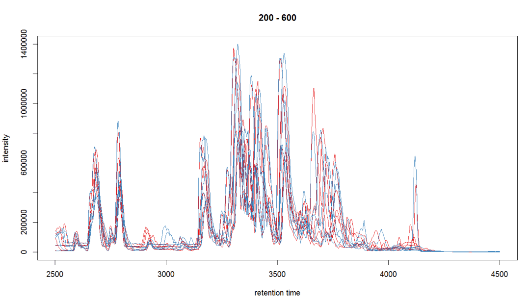
bpis <- chromatogram(raw_data, aggregationFun = "max") group_colors <- brewer.pal(3, "Set1")[1:2] names(group_colors) <- c("KO", "WT") plot(bpis, col = group_colors[raw_data$sample_group])

#查看某个个体

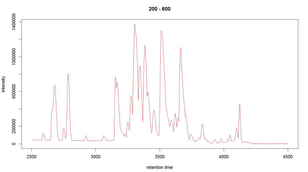
bpi_1 <- bpis[1, 1] plot(bpi_1, col = group_colors[raw_data$sample_group])

#查看样品离子流

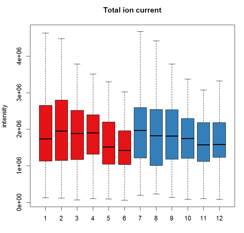
tc <- split(tic(raw_data), f = fromFile(raw_data)) boxplot(tc, col = group_colors[raw_data$sample_group],ylab = "intensity", main = "Total ion current")

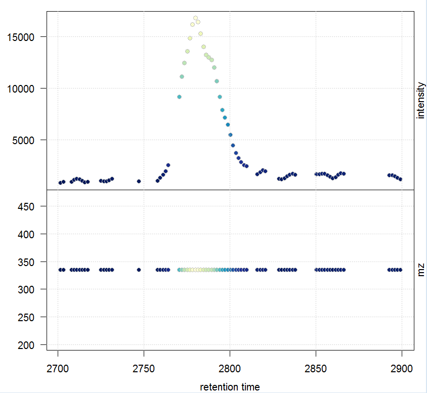
#定义保留时间与质荷比，提取特定的峰

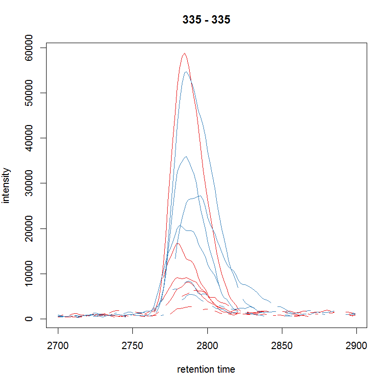
rtr <- c(2700, 2900) mzr <- c(334.9, 335.1) chr_raw <- chromatogram(raw_data, mz = mzr, rt = rtr) plot(chr_raw, col = group_colors[chr_raw$sample_group])

#提取质谱数据

msd_raw <- extractMsData(raw_data, mz = mzr, rt = rtr) plotMsData(msd_raw[[1]])

#定义峰宽与噪音，自动找出所有的峰

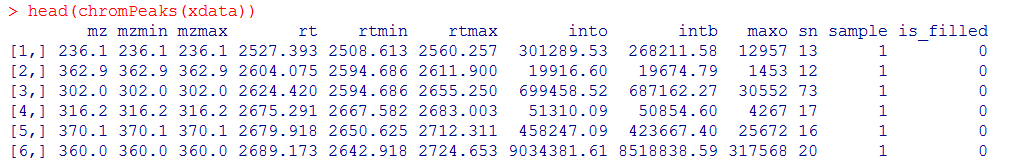
cwp <- CentWaveParam(peakwidth = c(30, 80), noise = 1000) xdata <- findChromPeaks(raw_data, param = cwp) head(chromPeaks(xdata))

#统计检测到的峰

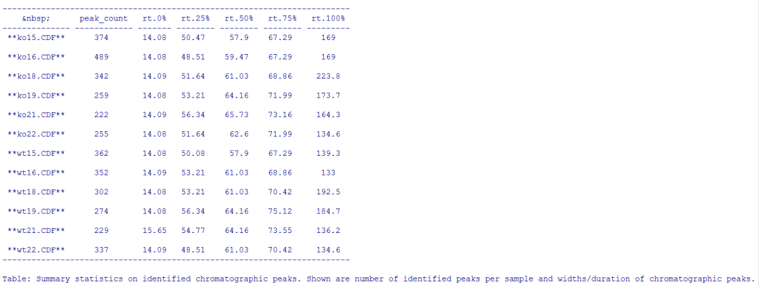
summary_fun <- function(z) { c(peak_count = nrow(z), rt = quantile(z[, "rtmax"] - z[, "rtmin"])) } T <- lapply(split.data.frame(chromPeaks(xdata), f = chromPeaks(xdata)[, "sample"]), FUN = summary_fun) T <- do.call(rbind, T) rownames(T) <- basename(fileNames(xdata)) pandoc.table(T, caption = paste0("Summary statistics on identified chromatographic", " peaks. Shown are number of identified peaks per", " sample and widths/duration of chromatographic ", "peaks."))

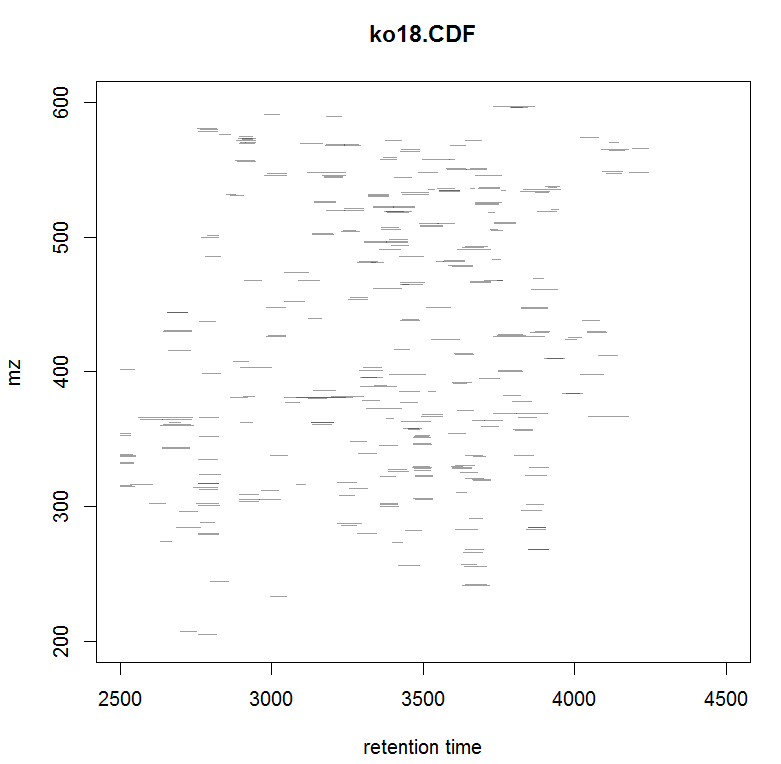
#画某个样品的峰图

plotChromPeaks(xdata, file = 3)

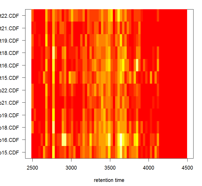
#对所有样品画热图

plotChromPeakImage(xdata)

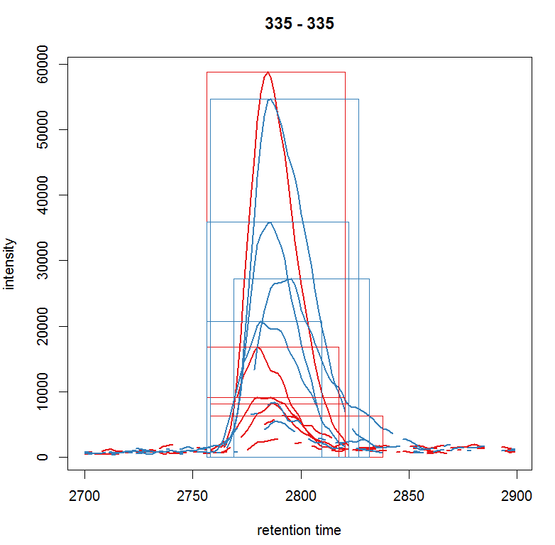
#标注某个峰的差异

plot(chr_raw, col = group_colors[chr_raw$sample_group], lwd = 2) highlightChromPeaks(xdata, border = group_colors[chr_raw$sample_group],lty = 3, rt = rtr, mz= mzr)

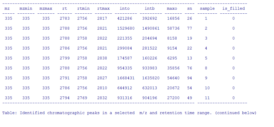
#提取某个峰所有样品的数据

pander(chromPeaks(xdata, mz = mzr, rt = rtr),caption = paste("Identified chromatographic peaks in a selected ","m/z and retention time range."))

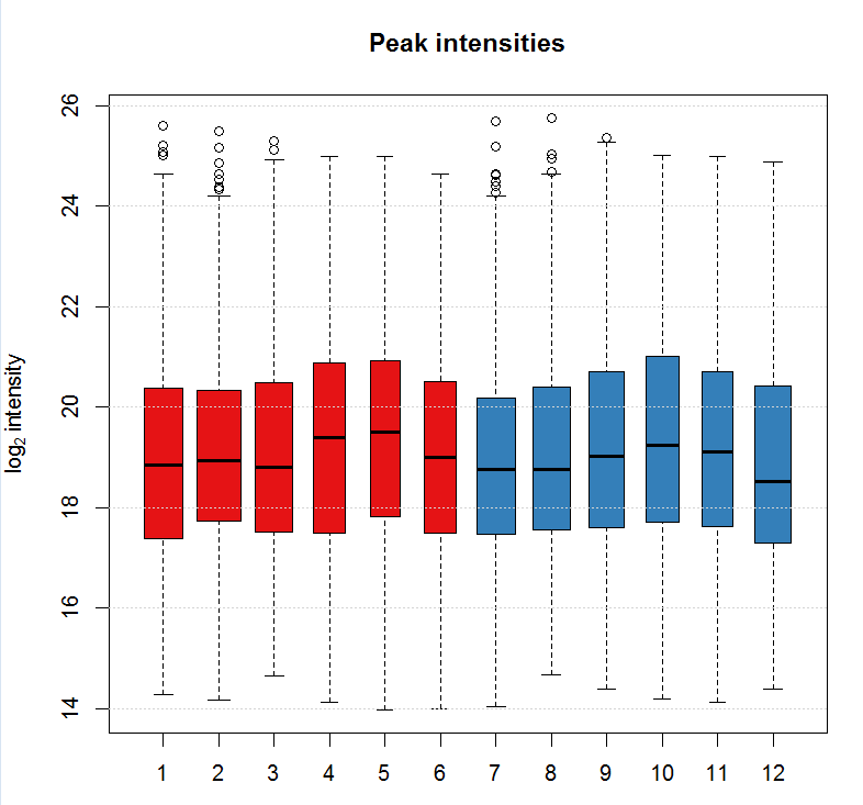
#画峰强的箱线图

ints <- split(log2(chromPeaks(xdata)[, "into"]),f = chromPeaks(xdata)[, "sample"]) boxplot(ints, varwidth = TRUE, col = group_colors[xdata$sample_group],ylab =expression(log[2]~intensity), main = "Peak intensities") grid(nx = NA, ny = NULL)

# 设定binSize

xdata <- adjustRtime(xdata, param = ObiwarpParam(binSize = 0.6))

#查看校正过的保留时间

head(adjustedRtime(xdata))

#查看校正前的保留时间

> head(rtime(xdata, adjusted = FALSE))

#画校正保留时间后的峰图及校正后与校正前的差异

bpis_adj <- chromatogram(xdata, aggregationFun = "max") par(mfrow = c(2, 1), mar = c(4.5, 4.2, 1, 0.5)) plot(bpis_adj, col = group_colors[bpis_adj$sample_group])

#查看数据是否校正过时间

hasAdjustedRtime(xdata) [1] TRUE

#恢复到没校正的状态

xdata <- dropAdjustedRtime(xdata) hasAdjustedRtime(xdata) [1] FALSE

#根据样品组设定参数

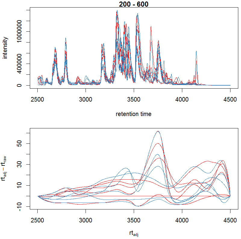
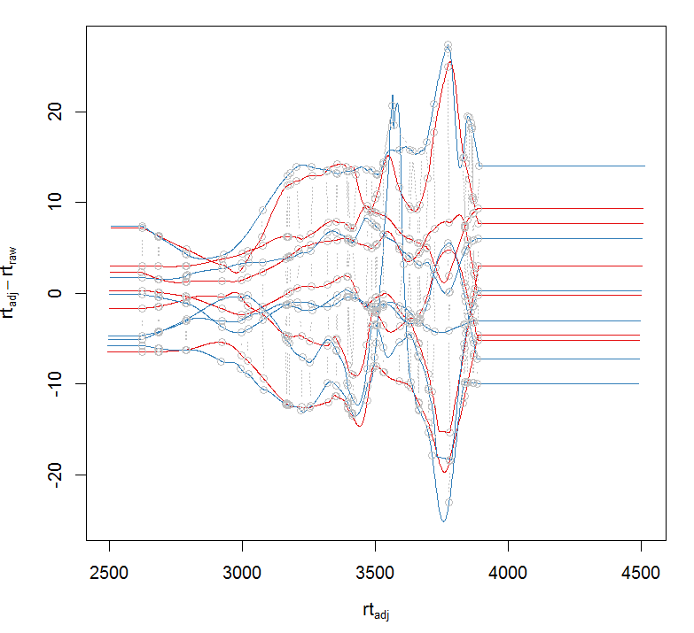
pdp <- PeakDensityParam(sampleGroups = xdata$sample_group,minFraction = 0.8) #根据组来提取数据 xdata <- groupChromPeaks(xdata, param = pdp) #根据组来校正时间 pgp <- PeakGroupsParam(minFraction = 0.85) xdata <- adjustRtime(xdata, param = pgp) #对校正前和校正后的结果作图 plotAdjustedRtime(xdata, col = group_colors[xdata$sample_group],peakGroupsCol = "grey", peakGroupsPch = 1)

#对校正前和校正后的某个峰作图

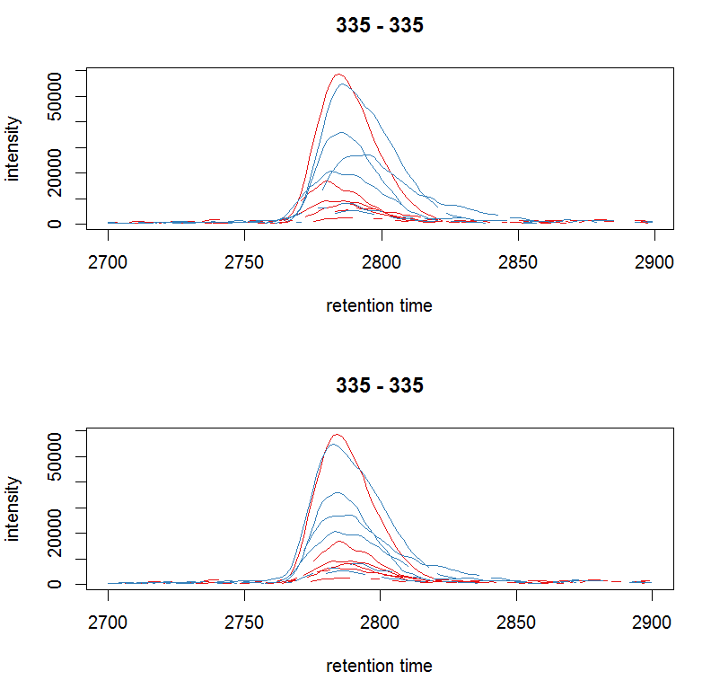
par(mfrow = c(2, 1)) plot(chr_raw, col = group_colors[chr_raw$sample_group]) chr_adj <- chromatogram(xdata, rt = rtr, mz = mzr) plot(chr_adj, col = group_colors[chr_raw$sample_group])

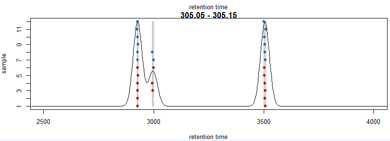
#选择一种质荷比，提取峰图

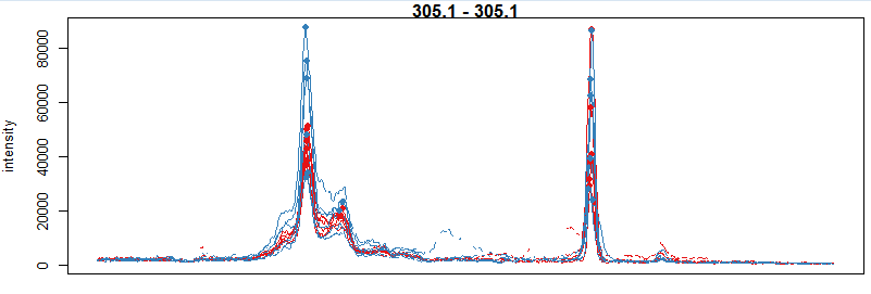
mzr <- c(305.05, 305.15) chr_mzr <- chromatogram(xdata, mz = mzr, rt = c(2500, 4000)) par(mfrow = c(3, 1), mar = c(1, 4, 1, 0.5)) cols <- group_colors[chr_mzr$sample_group] plot(chr_mzr, col = cols, xaxt = "n", xlab = "") highlightChromPeaks(xdata, mz = mzr, col = cols, type = "point", pch = 16)

#画一级质谱和二级质谱的峰图

mzr <- c(305.05, 305.15) chr_mzr_ms1 <- chromatogram(filterMsLevel(xdata, 1), mz = mzr, rt = c(2500, 4000)) plot(chr_mzr_ms1) chr_mzr_ms2 <- chromatogram(filterMsLevel(xdata, 2), mz = mzr, rt = c(2500, 4000)) plot(chr_mzr_ms2)

#定义峰提取参数

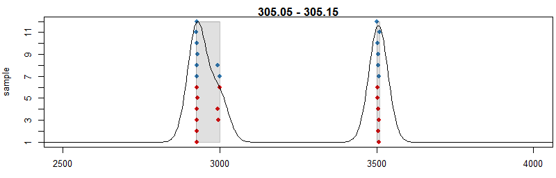
pdp <- PeakDensityParam(sampleGroups = xdata$sample_group,minFraction = 0.4, bw = 30) par(mar = c(4, 4, 1, 0.5)) plotChromPeakDensity(xdata, mz = mzr, col = cols, param = pdp,pch = 16, xlim = c(2500, 4000))

#用不同的峰提取参数，bw定义了距离多少的两个峰合并为一个峰

pdp <- PeakDensityParam(sampleGroups = xdata$sample_group,minFraction = 0.4, bw = 20) plotChromPeakDensity(xdata, mz = mzr, col = cols, param = pdp,pch = 16, xlim = c(2500, 4000))

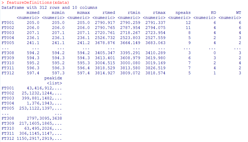
#提取数据，minFraction是占所有样本百分之多少以上的峰视为正确的数据

pdp <- PeakDensityParam(sampleGroups = xdata$sample_group,minFraction = 0.4, bw = 20) xdata <- groupChromPeaks(xdata, param = pdp) featureDefinitions(xdata)

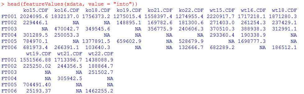
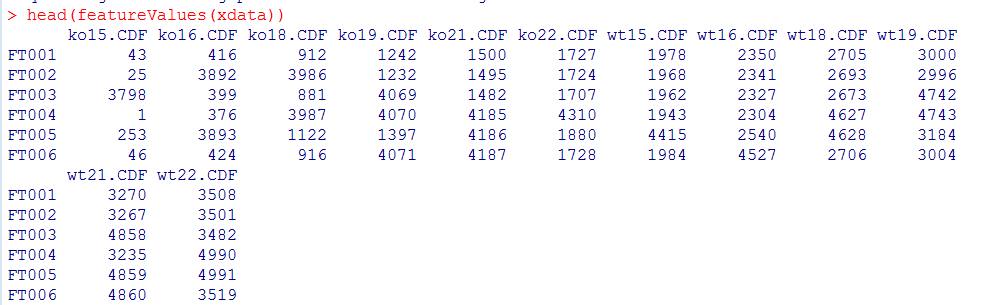
#对结果分组

head(featureValues(xdata, value = "into"))

#利用原始数据对NA进行回填

xdata <- fillChromPeaks(xdata)

head(featureValues(xdata))

#查看回填前的NA

apply(featureValues(xdata, filled = FALSE), MARGIN = 2,FUN = function(z) sum(is.na(z)))

#查看回填后的NA

apply(featureValues(xdata), MARGIN = 2,FUN = function(z) sum(is.na(z)))

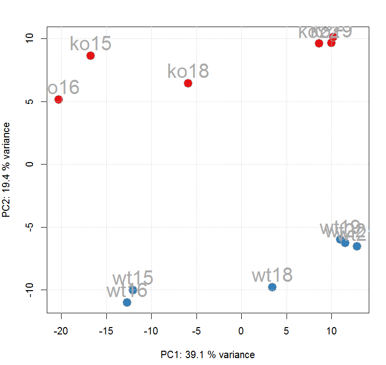
#PCA

ft_ints <- log2(featureValues(xdata, value = "into")) pc <- prcomp(t(na.omit(ft_ints)), center = TRUE) cols <- group_colors[xdata$sample_group] pcSummary <- summary(pc) plot(pc$x[, 1], pc$x[,2], pch = 21, main = "", xlab = paste0("PC1: ", format(pcSummary$importance[2, 1] * 100,digits = 3), " % variance"),ylab = paste0("PC2: ", format(pcSummary$importance[2, 2] * 100,digits = 3), " % variance"),col = "darkgrey", bg = cols, cex = 2) grid() text(pc$x[, 1], pc$x[,2], labels = xdata$sample_name, col = "darkgrey",pos = 3, cex = 2)

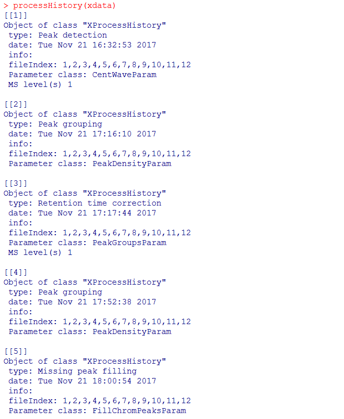
#查看数据处理历史，经过了Peak detection、Peak grouping、Retention time correction、Peak grouping、Missing peak filling

processHistory(xdata)

#提取某一步的数据

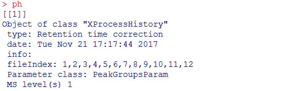
ph <- processHistory(xdata, type = "Retention time correction")

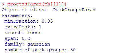
#提取数据的参数

processParam(ph[[1]])

#提取某个文件的数据

subs <- filterFile(xdata, file = c(2, 4))

#提取数据并留取保留时间

subs <- filterFile(xdata, keepAdjustedRtime = TRUE)

#按保留时间提取数据

subs <- filterRt(xdata, rt = c(3000, 3500))

range(rtime(subs))

#提取某个文件的所有数据

one_file <- filterFile(xdata, file = 3)

one_file_2 <- xdata[fromFile(xdata) == 3]

#查看峰文件

head(chromPeaks(xdata))

#导出数据

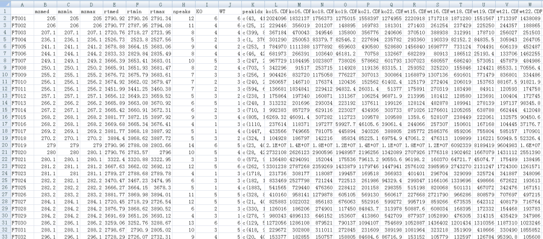
result<-cbind(as.data.frame(featureDefinitions(xdata)),featureValues(xdata, value = "into"))

write.table(result,file="xcms_result.txt",sep="\t",quote=F)

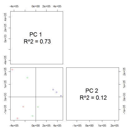
#PCA

values <- groupval(xdata) data <- t(values) pca.result <- pca(data) library(pcaMethods) pca.result <- pca(data) loadings <- pca.result@loadings scores <- pca.result@scores plotPcs(pca.result, type = "scores",col=as.integer(sampclass(xdata)) + 1)

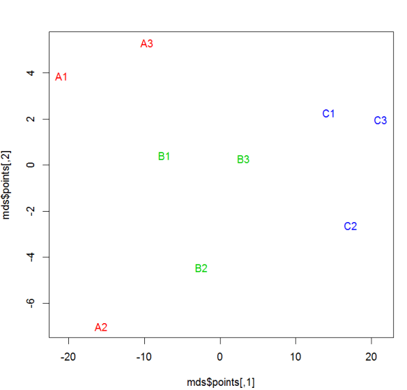
#MDS

library(MASS) for (r in 1:ncol(data)) data[,r] <- data[,r] / max(data[,r]) data.dist <- dist(data) mds <- isoMDS(data.dist) plot(mds$points, type = "n") text(mds$points, labels = rownames(data),col=as.integer(sampclass(xdata))+ 1 )