ChIP-seq主要用来研究蛋白质和DNA的相互作用,ChIPseeker 可以用来对ChIP-seq数据进行注释与可视化,下面我们就来介绍一下如何用ChIPseeker对chip-seq数据进行可视化操作。
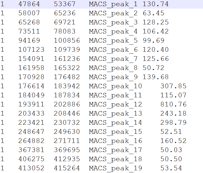
操作步骤把所有sample_peaks文件放在工作路径下,格式为
#安装程序
#source("http://bioconductor.org/biocLite.R") #biocLite("ChIPseeker") #biocLite("TxDb.Athaliana.BioMart.plantsmart28")#开始分析
library("ChIPseeker") library(ggplot2) library("TxDb.Athaliana.BioMart.plantsmart28") txdb <- TxDb.Athaliana.BioMart.plantsmart28 get_files_data<-function () { dir <- getwd() files <- list.files(dir) protein <- gsub(pattern = "GSM\\d+_(\\w+_\\w+)_.*", replacement = "\\1", files) protein <- sub("_Chip.+", "", protein) res <- paste(dir, files, sep = "/") res <- as.list(res) names(res) <- protein return(res)} files<-get_files_data()#读入启动子信息
promoter <- getPromoters(TxDb=txdb,upstream=3000, downstream=3000)#画覆盖图
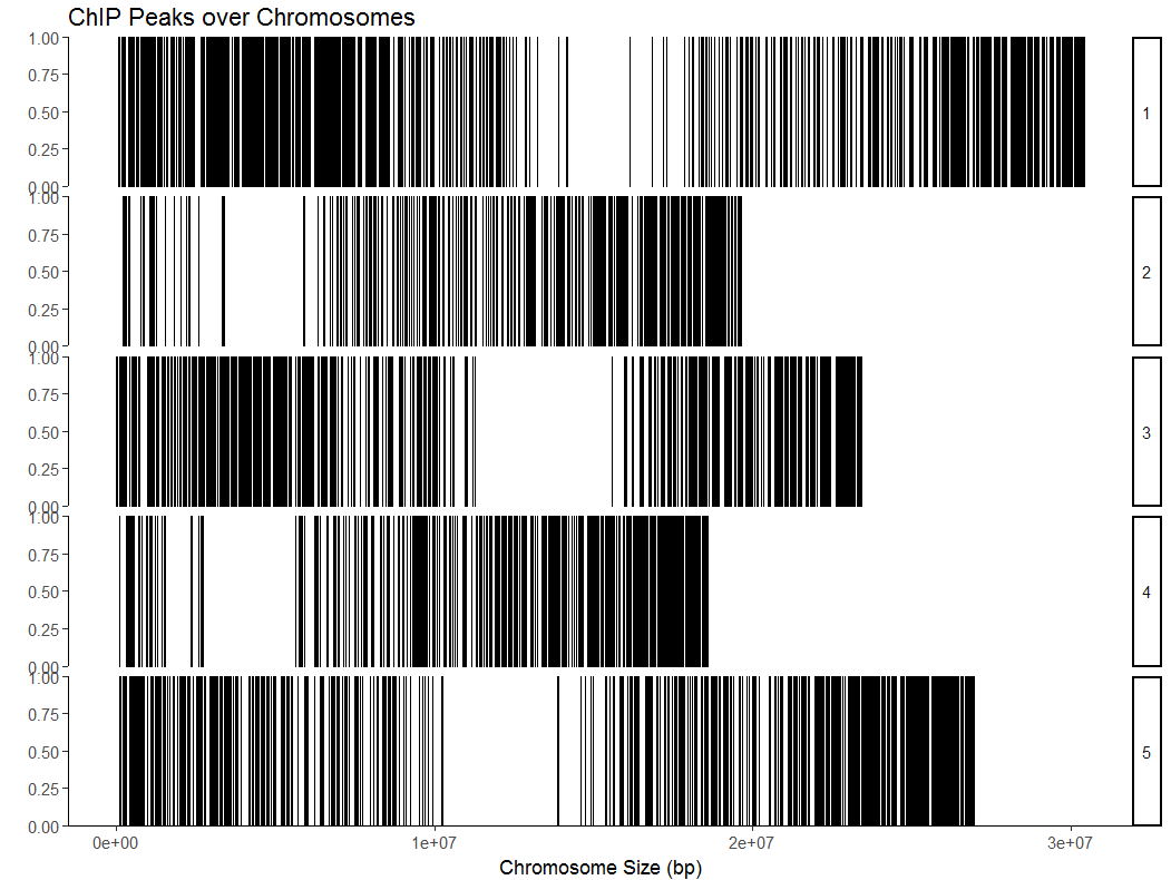
covplot(files[[4]])
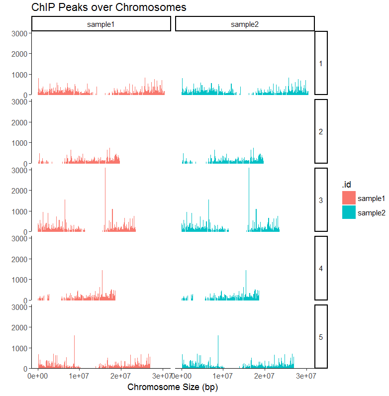
#画两个样品的覆盖图
peak1=GenomicRanges::GRangesList(sample1=readPeakFile(files[[1]]),sample2=readPeakFile(files[[2]])) covplot(peak1, weightCol="V5") + facet_grid(chr ~ .id)
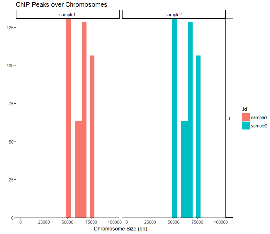
#放大一个区域
covplot(peak1, weightCol="V5", chrs=c("1", "2"), xlim=c(1, 100000)) + facet_grid(chr ~ .id)
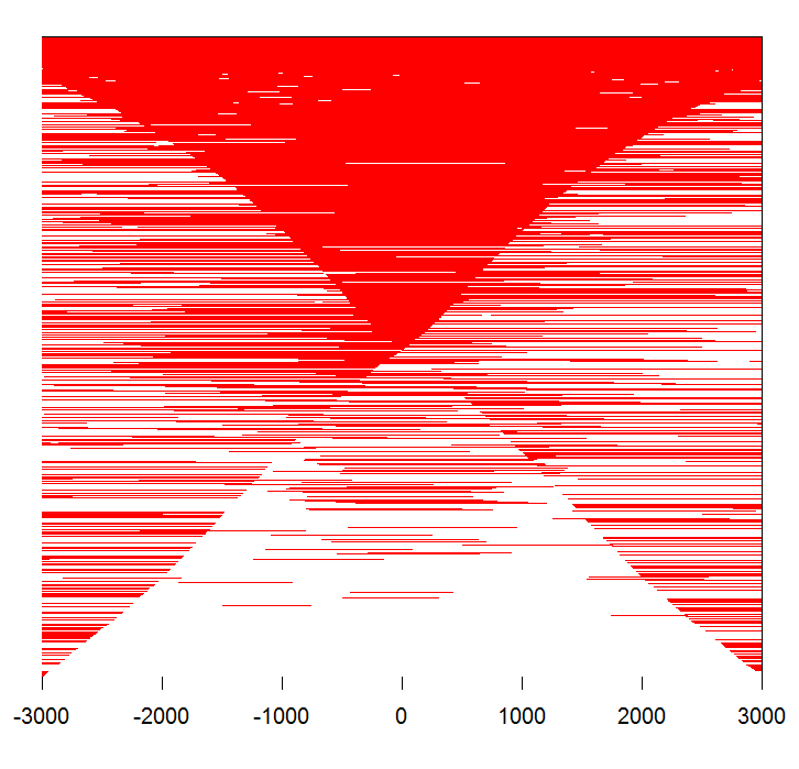
#画其中一个热图
peak <- readPeakFile(files[[4]]) tagMatrix <- getTagMatrix(peak, windows=promoter) tagHeatmap(tagMatrix, xlim=c(-3000, 3000), color="red")
#画结合区域热图
peakHeatmap(files,weightCol="V5",TxDb=txdb,upstream=3000,downstream=3000,color=rainbow(length(files)))
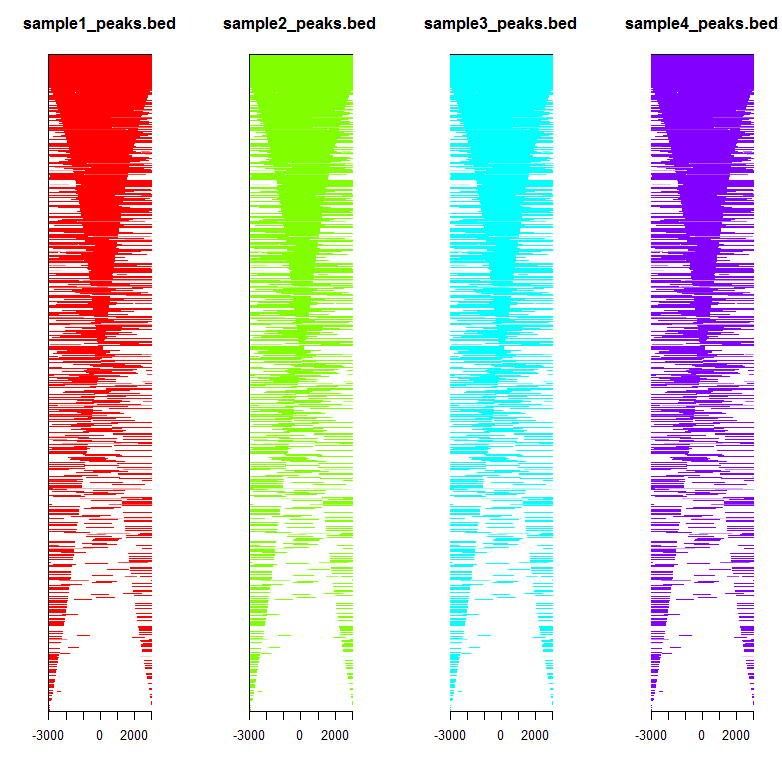
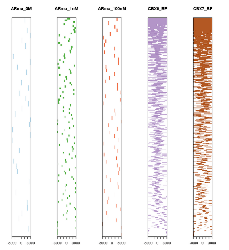
如图所示,前三个样品结合位点不在转录起始区域,后两个在。说明前三个样品不是调控转录的。
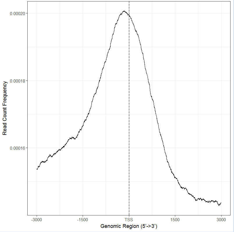
#结合强度图
plotAvgProf(tagMatrix, xlim=c(-3000, 3000),xlab="Genomic Region (5’->3’)",ylab = "Read Count Frequency")
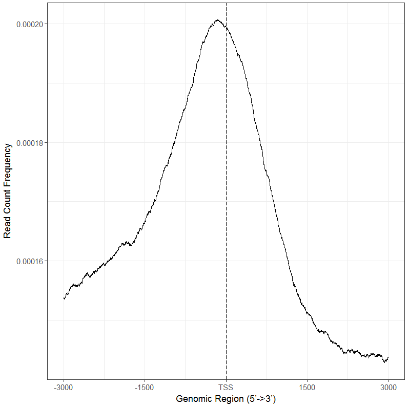
可以看到转录起始区域结合强度最高
#直接以文件做图,结果与上图一致
plotAvgProf2(files[[4]], TxDb=txdb,upstream=3000, downstream=3000,xlab="Genomic Region (5’->3’)",ylab = "Read Count Frequency")
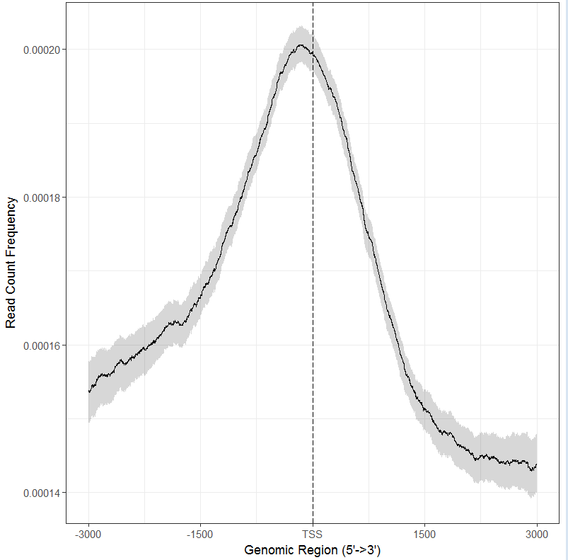
#加上bootstrap值
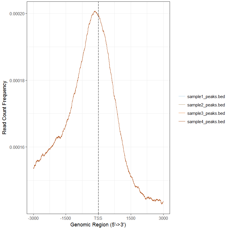
#所有数据一起做图
tagMatrixList <- lapply(files,getTagMatrix,windows=promoter) plotAvgProf(tagMatrixList, xlim=c(-3000, 3000))
#分面,同时计算置信区间
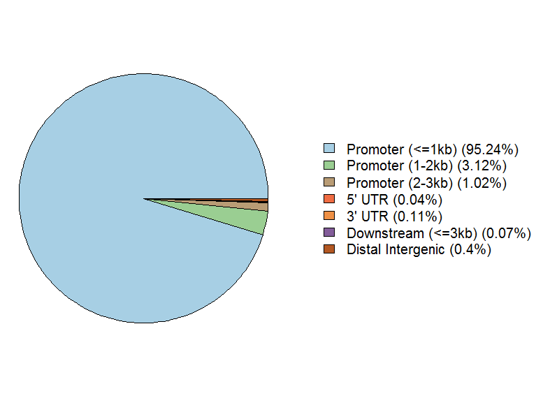
plotAvgProf(tagMatrixList, xlim=c(-3000, 3000),conf=0.95,resample=500, facet="row")#画饼状图
peakAnno <- annotatePeak(files[[4]], tssRegion=c(-3000, 3000),TxDb=txdb, annoDb="org.At.tair.db") plotAnnoPie(peakAnno)
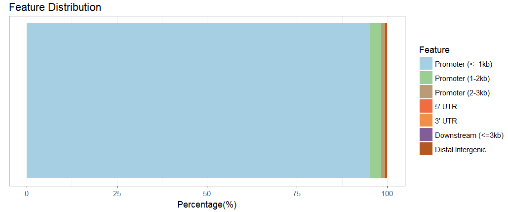
#画柱状图
plotAnnoBar(peakAnno)
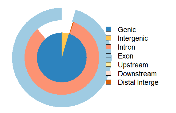
#画维恩饼图
vennpie(peakAnno)
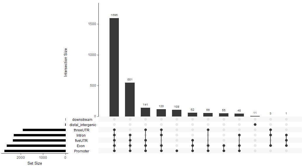
#画 upset图
upsetplot(peakAnno)
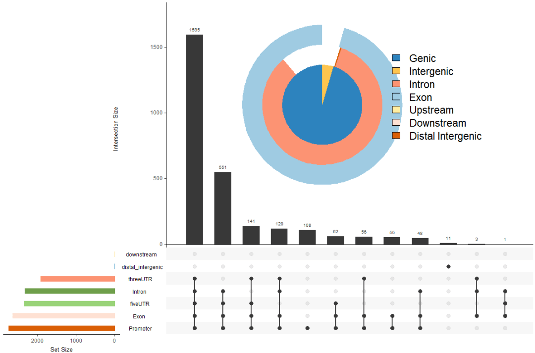
#结合起来
upsetplot(peakAnno, vennpie=TRUE)
#离最近基因的距离
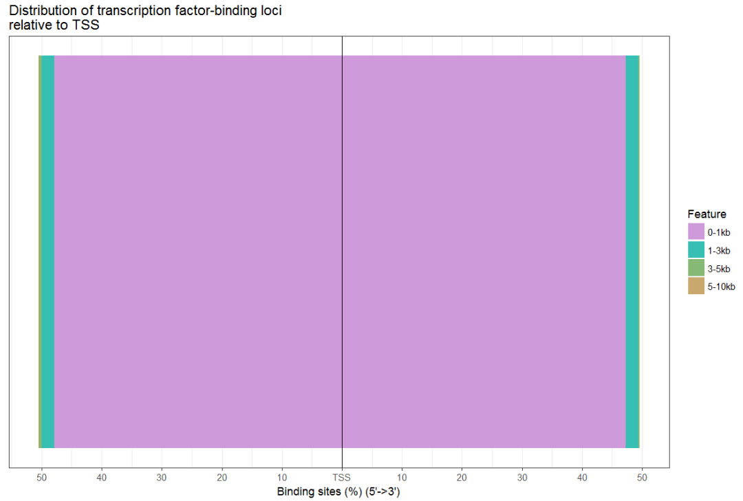
plotDistToTSS(peakAnno,title="Distribution of transcription factor-binding loci\nrelative to TSS")
#同时画多个柱状图
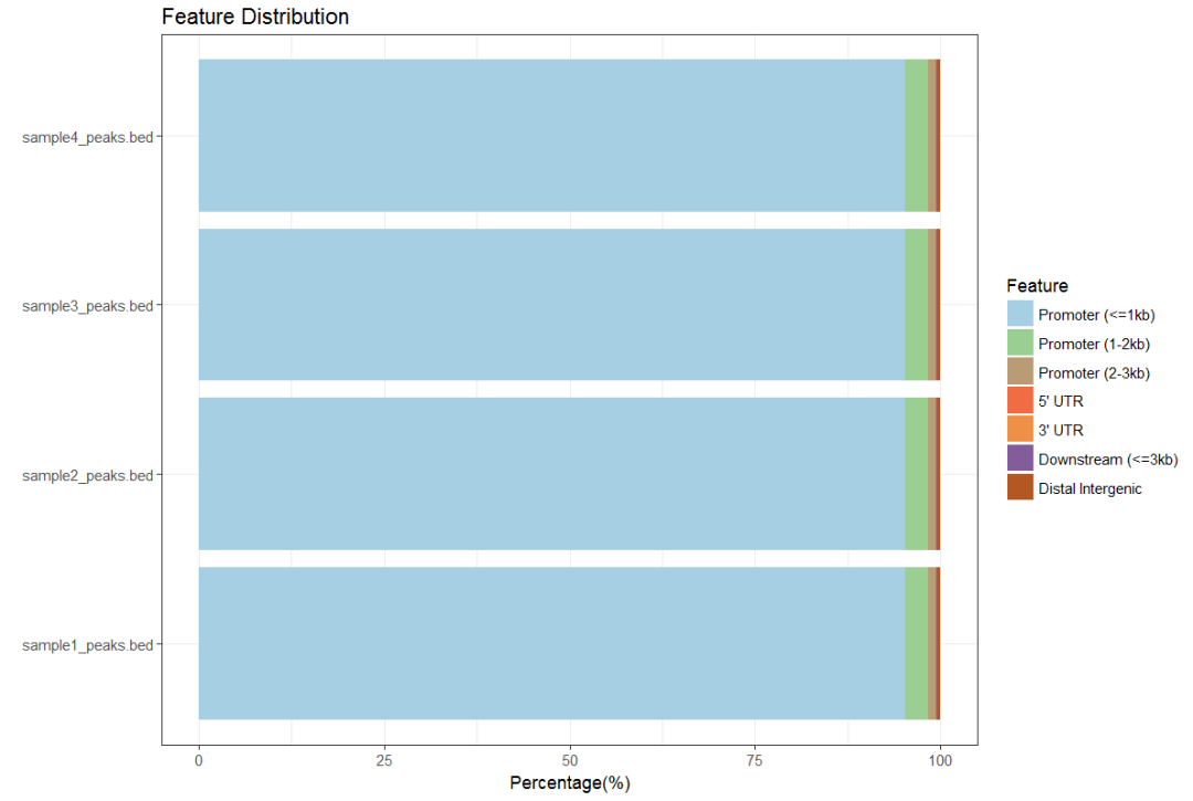
peakAnnoList <- lapply(files, annotatePeak, TxDb=txdb,tssRegion=c(-3000, 3000), verbose=FALSE) plotAnnoBar(peakAnnoList)
#同时画多个距离图
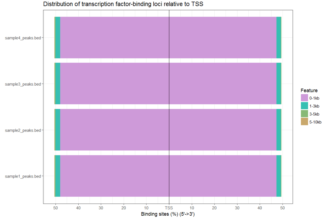
plotDistToTSS(peakAnnoList)
#画维恩图
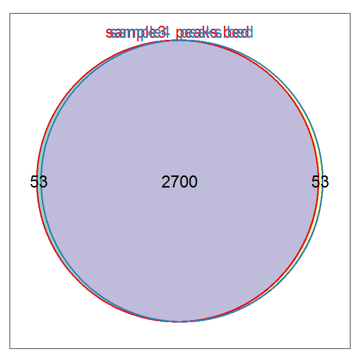
genes <- lapply(peakAnnoList, function(i)as.data.frame(i)$geneId) vennplot(genes[2:4], by="Vennerable")
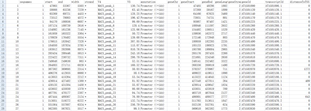
#输出注释信息
peakAnnotable<-as.data.frame(peakAnno) write.table(peakAnnotable,file="peakanno.result",sep="\t",quote=F)
- 本文固定链接: https://maimengkong.com/image/912.html
- 转载请注明: : 萌小白 2022年5月10日 于 卖萌控的博客 发表
- 百度已收录